A Signal is a Vector

A signal is usually stored as a long list of samples, but that list is rarely its most economical description. Choose the right basis — the right set of axes to measure it against — and nearly all of those numbers collapse to zero, leaving a sparse handful that describes the signal with almost no loss.

This post builds that idea from first principles, on a small signal.

1. A signal is a high-dimensional vector

Start with a real-world signal: a sound wave, a temperature trace, a row of pixel intensities. Almost any measurement unfolds over time or space.

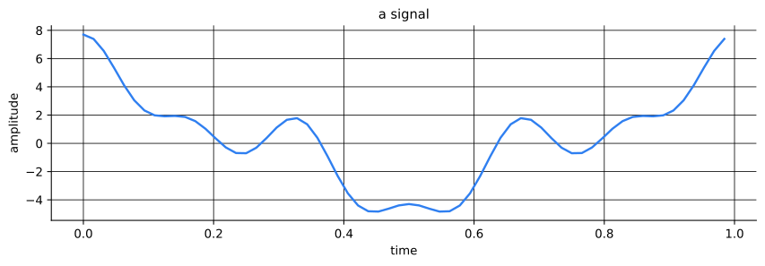
When we measure the signal, we sample its values at evenly spaced intervals — here $n=64$ of them.

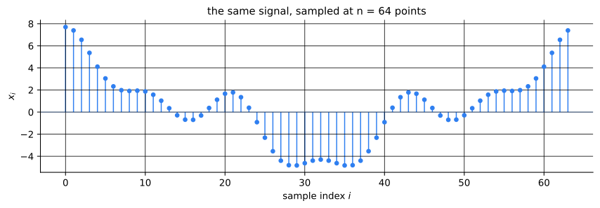
Stack those samples into a column and the signal becomes a single vector:

$$\mathbf{x}=\left[\begin{array}{c}{x}_1\\ x_2\\ ⋮\\ x_n\end{array}\right]\in {\mathbb{R}}^n.$$

The entire signal is a single point in an $n$-dimensional space. Each sample is its extent along one dimension. Our signal is one point in ${\mathbb{R}}^{64}$.

2. Changing coordinates

What happens if we change the coordinates — the basis vectors — we measure against?

Here is a two-dimensional vector $\mathbf{V}$ measured against two sets of axes: the standard basis in blue, and a rotated basis in red. Drag the slider. The arrow never moves. Only the numbers we measure it with do.

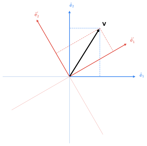
A vector is a geometric object — an arrow that exists before any axes are chosen. Selecting a basis only fixes the rulers we measure it against. Collect two orthonormal basis vectors ${\hat{\mathbf{e}}}_1^{\prime },{\hat{\mathbf{e}}}_2^{\prime }$ as the columns of a matrix,

$$B=\left[\begin{array}{cc}|& |\\ {\hat{\mathbf{e}}}_1^{\prime }& {\hat{\mathbf{e}}}_2^{\prime }\\ |& |\end{array}\right]$$

and that matrix is the transformation — here a rotation of the axes. The same vector $\mathbf{v}$ acquires new coordinates ${\mathbf{x}}^{\prime }$:

$$\mathbf{v}=B{\mathbf{x}}^{\prime },{\mathbf{x}}^{\prime }=B^{\top }\mathbf{v}.$$

Because the basis is orthonormal, $B^{\top }=B^{-1}$: the change of basis is a reversible rotation that discards nothing.

The same move in $n$ dimensions

Nothing about this is special to two dimensions. Choose any orthonormal basis of ${\mathbb{R}}^n$ — unit vectors ${\mathbf{\psi }}_1,\dots ,{\mathbf{\psi }}_n$ meeting at right angles — and collect them as the columns of a matrix $\Psi$. Just as $B$ turned a vector’s standard coordinates into rotated ones, $\Psi$ gives the same vector $\mathbf{x}$ new coordinates $\mathbf{s}={\Psi }^{\top }\mathbf{x}$:

$$\mathbf{x}=\Psi \mathbf{s}=\left[\begin{array}{cccc}|& |& & |\\ {\mathbf{\psi }}_1& {\mathbf{\psi }}_2& \cdots & {\mathbf{\psi }}_n\\ |& |& & |\end{array}\right]\left[\begin{array}{c}{s}_1\\ s_2\\ ⋮\\ s_n\end{array}\right]=\sum _{k=1}^n{s}_k{\mathbf{\psi }}_k.$$

Reading the product column by column, the signal is just a weighted sum of the basis vectors ${\mathbf{\psi }}_k$, each scaled by its coordinate $s_k$. Orthonormality (${\Psi }^{\top }\Psi =I$) keeps this a pure rotation: nothing is lost, and it reverses exactly through $\Psi$.

Parseval's theorem

An orthonormal rotation preserves length, $\Vert \mathbf{x}\Vert =\Vert \mathbf{s}\Vert$ — the signal carries the same energy in every such basis.

3. Bases of waves: Fourier and the DCT

For natural signals the most useful rotations use waves of increasing frequency as their axes. This is just another orthonormal basis, so its coordinates describe the same signal vector $\mathbf{x}$ as faithfully as the raw samples do. We have only rotated $\mathbf{x}$ into a more revealing frame.

Fourier

The Fourier basis writes a signal as a sum of complex exponentials of increasing frequency,

$${\mathbf{\psi }}_k\propto e^{2\pi ikt}=\cos (2\pi kt)+i\sin (2\pi kt),$$

where Euler’s formula unpacks each exponential into a cosine and a sine. Paired with the fast Fourier transform, this single decomposition became the backbone of modern signal processing — audio and image coding, communications, filtering, and spectral analysis all live in it.

The DCT

Splitting each complex exponential into its cosine and sine parts gives a real Fourier basis: a constant DC term, then a normalized cosine/sine pair at each frequency $k$,

$${\mathbf{\psi }}_1=\frac{1}{\sqrt{n}}1,{\mathbf{\psi }}_k^{\cos }=\sqrt{\frac{2}{n}}\cos (2\pi kt),{\mathbf{\psi }}_k^{\sin }=\sqrt{\frac{2}{n}}\sin (2\pi kt).$$

The discrete cosine transform (DCT), introduced by Nasir Ahmed in 1974, goes one step further and keeps only the cosines. An even reflection of the signal at its edges avoids the artificial jump a periodic basis imposes at the boundary, and its energy-compacting cosines made it the workhorse behind JPEG, MPEG, and MP3 — among the most widely used transforms in computing. Each column is a single cosine of rising frequency,

$${\mathbf{\psi }}_k(i)\propto \cos \left(\frac{\pi (2i+1)k}{2n}\right),$$

with the $k=0$ column normalized by $\sqrt{1/n}$ and the rest by $\sqrt{2/n}$.

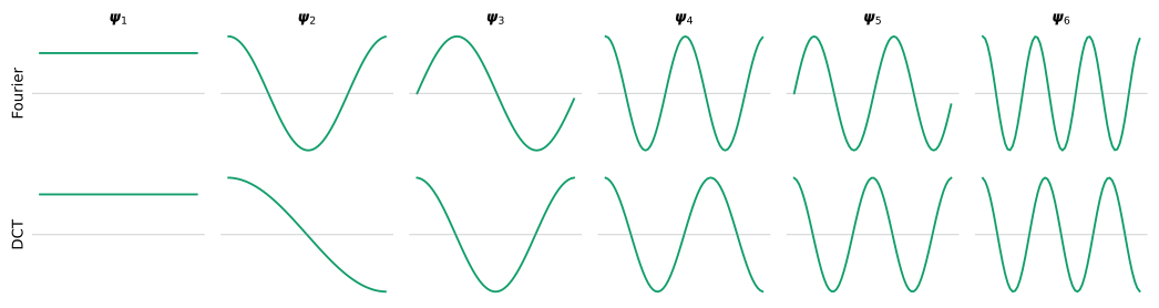
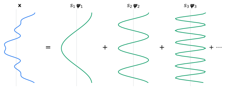
A coordinate $s_k={\mathbf{\psi }}_k^{\top }\mathbf{x}$ asks how much of wave $k$ is present in the signal. Each column of $\Psi$ — Fourier or DCT — is one wave; the first six of each are plotted below.

4. Building the signal one wave at a time

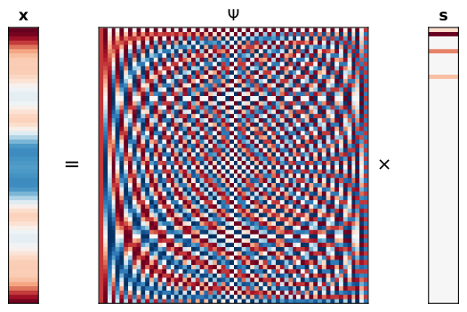
A change of basis is a recipe for rebuilding the signal: stack the basis waves as the columns of $\Psi$, weight each by its coordinate $s_k$, and sum.

$$\mathbf{x}=\Psi \mathbf{s}=\sum _k{s}_k{\mathbf{\psi }}_k.$$

The same statement as matrices: a tall column $\mathbf{x}$, the square basis $\Psi$, and the coordinate column $\mathbf{s}$.

5. The payoff: the right basis is sparse

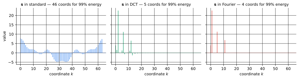
Below is the same $64$-dimensional signal expressed in three bases. In the standard basis all $64$ coordinates matter. Rotated into the DCT, the energy concentrates in a few low-frequency coordinates. Rotated into the Fourier basis — exactly matched to this periodic signal — all but a handful of coordinates are zero:

$${\mathbf{s}}_{\text{Fourier}}\approx [\underset{\text{a few}}{\underbrace{s_1,\dots ,s_r}},0,\dots ,0{]}^{\top }.$$

Same vector, same information, now described by $r\ll n$ numbers. That is sparsity. Beneath each panel is the number of coordinates needed to hold $99\%$ of the signal’s energy.

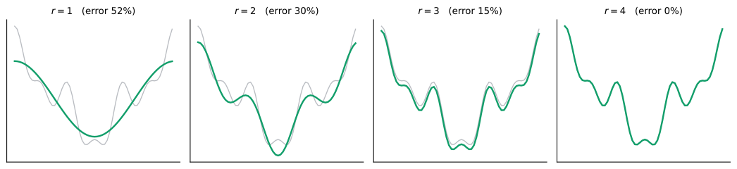
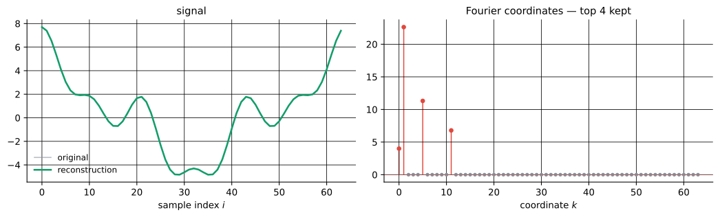
Those few nonzero coordinates are all it takes. Adding the Fourier waves back in order of importance — and because this signal is only a few Fourier cosines — a handful of terms does not merely approximate it. It reproduces it exactly:

6. Keep the top $r$

When most coordinates are near zero, discard them. Keep the $r$ largest, set the rest to zero to form ${\mathbf{s}}_r$, and rotate back:

$$\hat{\mathbf{x}}=\Psi {\mathbf{s}}_r.$$

In the Fourier basis the error collapses to zero at $r=4$; in the DCT it fades more gradually. The basis that matches the signal wins.

That is the whole idea behind transform coding. JPEG does exactly this to $8\times 8$ blocks of pixels in the DCT basis; MP3 does it to short windows of audio. The work is in choosing a basis where natural signals are sparse — and in the next post, in what happens when you don’t get to choose which coordinates you measure.

---

The figures and numerics here are generated from notebooks/01_signal_is_a_vector.py; the transforms are ported to TypeScript and parity-tested against scipy.